A heightmap looks like terrain data, but it is still only a 2D array of samples. By itself, it does not tell a renderer where the surface is, how the cells connect, or how the result should curve around a planet. Those decisions turn sample values into a mesh, and that is the point where a terrain system starts behaving like geometry instead of an image.

The same height values can become a small local patch, a streamed flat world, or a spherical planet. That is why this topic is worth slowing down for: the representation you choose determines how much detail survives, how expensive the mesh is to draw, and whether the result can wrap cleanly around a globe.

The first step is simple enough to see directly.

A Heightmap Is Not Yet Geometry

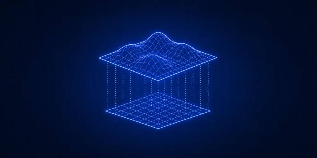
The left side of the visualization makes the source data concrete. You can move across the grid and see one selected cell light up, along with the four sample points at its corners. Those points are the important part, because the mesh does not come from the colored image itself. It comes from the sampled values at grid intersections.

Once those samples are turned into vertices, each rectangular cell becomes two triangles. That is the basic indexed-mesh pattern used in many terrain systems. If a heightmap has w columns and h rows, then the full grid produces w × h vertices and 2(w - 1)(h - 1) triangles before any optimization. The exact numbers matter less than the structure: vertices are shared, cells are split consistently, and the result is one continuous surface instead of a pile of disconnected quads.

This is the same core idea used in the classic CPU path described in LearnOpenGL’s height map walkthrough. The heightmap itself stays regular and rectangular. The mesh is the separate structure that makes the data renderable.

Two implementation details sit underneath that simple picture. First, the index buffer lets neighboring cells reuse the same corner vertices instead of duplicating them. Second, the triangle winding has to stay consistent so the renderer knows which side of each triangle is the front face. That is why the shared corner highlight matters in the visualization: it shows that the grid is not just a set of pixels, but a connectivity map for geometry.

If you want the upstream source of those height values, the article on Noise Functions: Value Noise, Perlin Noise, and Fractal Noise explains how a height signal is usually generated before it ever reaches a mesh builder.

A Flat Terrain Patch Is Just a Regular Mesh

Once the sample grid becomes vertices and triangles, the next step is placement. The simplest terrain is still just a subdivided plane with each vertex lifted vertically by its sample value. That is why the flat-terrain view is useful: it shows that “terrain” is not a special object type. It is a mesh whose shape changes because the vertex positions change.

The right side of the first visualization already shows that patch in perspective. Drag it and the view changes, but the underlying topology does not. That is the real lesson. The mesh stays a grid whether the surface looks smooth, steep, or gently rolling. The height values only move the vertices up and down; they do not change how the triangles are connected.

This separation explains why lighting matters so much. A flat terrain patch only looks convincing when the shading follows the slope of the surface. The normals are not stored in the heightmap image itself. They are derived from the shape of the mesh, either from neighboring height samples or from the triangle geometry after the mesh is built. When the light moves, you see the slope more clearly, because the bright and dark regions are responding to surface orientation rather than to the grayscale image on its own.

That is the same basic vertex-versus-shading split described in Vertex and Fragment Shaders in the Graphics Pipeline. The terrain mesh provides the geometry. The shader pipeline decides how that geometry is transformed and lit. In other words, heightmap conversion is only half of terrain rendering; the rest is the visual treatment that makes the surface readable from a camera.

For a simple local patch, a fixed-resolution grid is often enough. It is predictable, easy to stream, and easy to reason about. For a large world, though, the question becomes how much detail you can afford to keep everywhere.

Sampling Density Controls What Survives

The next visualization isolates that trade-off. It keeps the terrain shape and the probe position tied together, but changes the sampling density so the difference in detail is impossible to ignore.

The sparse mesh is cheaper, but it can flatten a hilltop, turn a ridge into a broad ramp, or erase a shallow basin entirely. The fine mesh keeps those shapes closer to the source data, but it pays for that accuracy with more vertices, more triangles, and more work every time the terrain is built or updated. The point is not that dense sampling is always better. The point is that detail has a cost, and terrain systems have to choose where that cost is worth paying.

That trade-off is one reason terrain engines rarely use one fixed grid everywhere. Instead, they vary resolution with distance or screen importance. The classic geometry-clipmap approach in Terrain Rendering Using GPU-Based Geometry Clipmaps keeps dense geometry near the viewer and coarser geometry farther away. NVIDIA’s Terrain Tessellation whitepaper makes the same practical point from a different angle: surface detail can be generated where the camera needs it instead of stored uniformly everywhere.

That is the practical meaning of level of detail in this context. It is not a separate topic from mesh generation. It is mesh generation with a budget. If the grid is too sparse, the mesh no longer matches the terrain signal. If the grid is too dense, the terrain becomes more expensive than the scene needs.

This is also where the article on Marching Cubes becomes a useful comparison. Marching Cubes also turns sampled data into geometry, but it starts from a volume rather than a heightfield. If you need caves, overhangs, or internal structure, a heightmap is usually the wrong representation.

A Spherical World Needs a Different Layout

Flat terrain is only one way to use a heightmap. For a planet, the same kind of data has to live on a curved surface, which changes the problem from “how do I lift this grid?” to “how do I place this grid on a sphere without breaking the poles?”

The lat/long view shows the familiar trap. It is easy to picture, but it squeezes too much area near the poles and creates a seam where the map wraps around. The cube-sphere view replaces that with face-based patches. Each face still uses a grid of samples, but the grid is distributed across six sides instead of being forced into one singular rectangular map.

That change solves the biggest geometric problem. It is not that the height values are different. It is that the coordinate system is better suited to a sphere. The same source terrain can wrap around the globe cleanly because the layout avoids the pole distortion that a single latitude/longitude grid creates.

This is why the research sources point to cube-to-sphere mapping papers and to projection systems such as the quadrilateralized spherical cube documentation. The exact spherical layout can vary, and some systems use HEALPix-style partitions instead, but the teaching point stays the same: the data can still be a heightmap, yet the surface representation has to match the shape of the world.

The face seams also reveal another practical rule. Adjacent patches must agree at their boundaries. If one face samples the edge differently from the next face, the globe will show cracks. So even when the planet is built from multiple patches, the edge samples and normals have to be coordinated as if they belonged to one continuous surface.

How the Pieces Fit Together

The mesh pipeline for a heightmap is really a sequence of representation choices:

1. take a 2D sample grid as input
2. turn each sample into a shared vertex
3. split each cell into triangles with consistent winding
4. derive normals so lighting follows the slope
5. choose a sampling density that matches the needed detail
6. choose a surface layout that matches the world shape

Those steps sound mechanical, but they control most of the visual result. The same heightmap can read as a small patch, a large open world, or a planet depending on how those choices are made. That is also why the topic connects naturally to the rest of the rendering pipeline. Once the mesh exists, vertex and fragment shaders determine how it is transformed and shaded. Once the data becomes volumetric instead of height-based, signed distance fields and Marching Cubes become more relevant conversion paths.

The practical takeaway is simple. A heightmap is not terrain in the visual sense until the mesh pipeline decides what to do with it. The surface you see is the result of several small decisions, and each decision has a visible consequence:

• shared vertices prevent cracks
• triangle winding keeps the surface oriented correctly
• normals make the slope readable
• higher density preserves more detail
• spherical layouts avoid pole distortion

If you keep those five ideas in view, heightmap conversion stops feeling like a black box. It becomes a clear chain from sampled values to renderable terrain.