Bezier curves are one of the most common tools for drawing smooth paths in computer graphics, UI motion, vector illustration, and font rendering. Even when a curve looks freehand, many systems represent it with a small set of control points and a deterministic equation. That makes Bezier curves both expressive and reliable: artists and engineers can shape motion and geometry with only a few values.

This article builds a practical understanding from the ground up. You will start with the quadratic case, connect handle placement to tangent direction, compare quadratic and cubic handle behavior directly, and then inspect how De Casteljau’s algorithm computes points on either kind of curve. Before getting into notation, start with the basic behavior: one movable handle changes a smooth curve between two fixed endpoints.

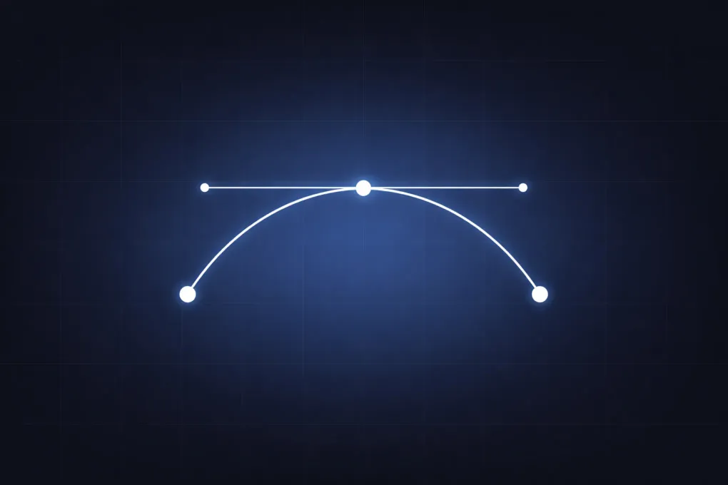
Drag the blue handle to reshape the curve while the two dark endpoints stay fixed. The dashed control polygon shows the straight-line structure that steers the smooth path. Moving the handle farther from the endpoint segment creates a stronger arch, while moving it closer makes the curve flatter.

Bezier Curve Control Points

A Bezier curve is defined by control points. The curve starts at the first control point and ends at the last control point. The points in between usually are not on the curve. Instead, they pull the curve direction and how much it bends. Bezier curves come in several forms, but this article focuses on the most common one: polynomial Bezier curves. In that family, the number of control points determines the degree of the curve. The control polygon is the sequence of straight segments connecting those points. It is not the rendered curve, but it is the easiest way to read how the curve will leave the start point, bend through the interior, and arrive at the end point.

The most common cases are quadratic and cubic Bezier curves. For a quadratic Bezier curve, there are three points:

• $P_0$: start point
• $P_1$: control point
• $P_2$: end point

For a cubic Bezier curve, there are four points:

• $P_0$: start point
• $P_1$: first handle
• $P_2$: second handle
• $P_3$: end point

Those interior control points usually act like handles rather than points that the curve must pass through. Moving a handle changes tangent direction and bend strength while the endpoints remain fixed. That is the practical reason Bezier curves are useful in drawing tools, animation paths, and fonts: a small point set gives predictable smooth geometry.

Quadratic Bezier Curve Formula

A quadratic Bezier curve uses three control points and one parameter $t$. The formula uses a parameter $t$ from $0$ to $1$:

$$B(t) = (1 - t)^2 P_0 + 2(1 - t)t P_1 + t^2 P_2$$

You can read this as a weighted combination of points. At $t = 0$, all weight is on $P_0$, so the curve point is at the start. At $t = 1$, all weight is on $P_2$, so the curve point is at the end. Between them, weight shifts smoothly and produces a continuous path.

That smooth behavior comes from the fact that the weights are polynomials in $t$. As $t$ changes, the point on the curve moves continuously instead of jumping from one location to another.

Quadratic Shape Exploration

The same editable curve is worth revisiting now that the point labels have meaning. This is the simplest Bezier shape: two fixed endpoints and one movable control point. The curve starts at $P_0$, ends at $P_2$, and bends toward $P_1$. As the blue $P_1$ handle moves, the control polygon shows the straight-line scaffold while the curve shows the smoothed result. Pulling $P_1$ far away from the segment from $P_0$ to $P_2$ makes the path arch strongly; bringing it back toward that segment flattens the curve without moving either endpoint.

The curve usually does not pass through $P_1$. Instead, the two segments connected to $P_1$ set the directions at the start and end of the curve. Moving the handle therefore changes both the amount of bend and the way the curve leaves $P_0$ and settles into $P_2$. This is why Bezier curves are useful: you can steer shape indirectly and keep smoothness. Those same ideas also lead to formal properties such as convex-hull containment and affine invariance, which the Michigan Tech construction notes explain in more detail.

Cubic Bezier Curve Formula

Most design and web tools prefer cubic Bezier curves. A cubic has four control points:

• $P_0$: start
• $P_1$: first handle
• $P_2$: second handle
• $P_3$: end

Its equation is:

$$B(t) = (1 - t)^3 P_0 + 3(1 - t)^2 t P_1 + 3(1 - t)t^2 P_2 + t^3 P_3$$

Compared to quadratic, cubic adds one more handle and much more shape control. You can create S-curves, gentle transitions, or aggressive turns without chaining multiple segments too early. That extra freedom also introduces behavior that quadratic curves cannot express, including inflection points and, in some control-point arrangements, cusp-like or self-intersecting shapes.

The comparison view makes the extra cubic handle visible as a control difference, not just a higher-degree equation. In the quadratic panel, dragging the single interior handle changes the whole arc and couples the start and end tangent directions. In the cubic panel, moving $P_1$ mostly changes the departure from $P_0$, while moving $P_2$ mostly changes the arrival into $P_3$. The shared Sample position slider connects that geometric behavior to the basis weights: three quadratic weights trade off across the span, while four cubic weights overlap and give the interior of the curve more freedom.

Pulling the two cubic handles to opposite sides of the chord from $P_0$ to $P_3$ shows the practical payoff. The endpoints stay fixed, but the curve can develop an S-shape because the two handles steer different parts of the segment. Quadratic curves are simpler and often enough for one arching bend, while cubic curves let you tune departure and arrival more independently. That local-handle behavior is the reason vector editors expose tangent handles for anchors. Each segment can be tuned without redrawing the full path manually. If you want to go further into these qualitative cubic shape changes, Pomax covers inflections and classification in more depth, and the Berkeley report on detecting cusps and inflection points in curves shows how those features follow from derivative structure rather than editor quirks. If you want to see the same curve idea extended into space, the companion article on visualizing 3D Bezier curves and De Casteljau construction shows how the control polygon, sampled path, and interpolation ladder behave under camera rotation.

Tangents and Motion Direction

Bezier curves are often used for motion paths, not just static drawings. The cubic handle view above makes the endpoint tangent idea easy to see. In animation, the local tangent direction matters because it tells you where an object is moving at that instant.

For a cubic curve, the derivative is:

$$B'(t) = 3(1 - t)^2 (P_1 - P_0) + 6(1 - t)t (P_2 - P_1) + 3t^2 (P_3 - P_2)$$

Two practical facts follow:

• At the start ($t = 0$), direction aligns with $P_1 - P_0$.
• At the end ($t = 1$), direction aligns with $P_3 - P_2$.

This is why moving the two interior control points changes how the curve leaves and approaches the endpoints. In vector and motion-path editors, those tangent directions are exposed as direction handles at the endpoints, so dragging them changes how the path departs and arrives.

When motion must feel natural, path geometry alone is not enough. You also need a timing function for how $t$ changes over time. A path can be smooth while speed still feels abrupt if the parameter progression is not eased.

De Casteljau Algorithm

The polynomial equations are compact, but there is another way to evaluate both quadratic and cubic Bezier curves: De Casteljau’s algorithm. It computes a point on the curve using repeated linear interpolation, which means every step has the same simple form: move a fraction $t$ of the way from one point to another. That is easier to inspect and debug than a larger polynomial expression because each intermediate point has a clear geometric meaning.

For the quadratic case at a chosen $t$:

1. Interpolate between $P_0$ and $P_1$ to get $Q_0$.
2. Interpolate between $P_1$ and $P_2$ to get $Q_1$.
3. Interpolate between $Q_0$ and $Q_1$ to get $B(t)$.

The final point is the same as the quadratic formula because linear interpolation is itself a weighted sum. If $Q_0 = (1 - t)P_0 + tP_1$ and $Q_1 = (1 - t)P_1 + tP_2$, then interpolating between them gives:

$$(1 - t)Q_0 + tQ_1 = (1 - t)^2 P_0 + 2(1 - t)t P_1 + t^2 P_2$$

That right-hand side is exactly the quadratic Bezier equation from the formula section above. The advantage is that this interpolation procedure extends naturally to higher degree curves and is numerically stable in many implementations. That matters because the same geometric procedure works for both the quadratic curve and the cubic curve.

In Quadratic mode, the interpolation slider shows how one curve point is built for each value of $t$. As $t$ moves from 0.00 to 1.00, $Q_0$ slides between $P_0$ and $P_1$, $Q_1$ slides between $P_1$ and $P_2$, and the final interpolated point traces the actual curve. Switching to Cubic mode adds one more interpolation round, but it does not add a new kind of operation: each point is still a linear blend between two points from the previous round.

This ladder view gives an immediate geometric reason for why the curve stays inside the convex region formed by the control points. It also shows why De Casteljau is useful for subdivision, which means splitting one Bezier segment into two smaller Bezier segments at the current value of $t$. The left half can be built from the points along one side of the interpolation ladder, and the right half can be built from the points along the other side. Rendering code uses that split when a curve is too bent to draw accurately with one straight segment: it keeps subdividing until each smaller piece is flat enough to approximate. The same operation is useful in adaptive tessellation and hit-testing. For a deeper visual treatment of splitting, derivatives, and subdivision, A Primer on Bezier Curves remains one of the strongest practical references.

Piecewise Bezier Paths and Continuity

Real drawings are usually not a single curve. They are chains of Bezier segments. When connecting segments, continuity is the main quality concern. Each segment may be smooth internally, but the shared anchor between two neighboring segments can still create a corner, a change in speed, or a sudden change in bending. The continuity label describes what agrees exactly at that one join.

Four useful continuity levels show up in practice:

• $C_0$ continuity: segments meet at the same point.
• $G_1$ continuity: tangent directions match, so the join looks smooth.
• $C_1$ continuity: first derivatives match, so direction and tangent magnitude are continuous.
• $C_2$ continuity: second derivatives match, so curvature changes smoothly.

The distinction between $G_1$ and $C_1$ is easy to miss because both can remove the visible corner. For a cubic segment, the tangent at the end points along the line from the last handle into the endpoint, and the tangent at the next segment points from the shared endpoint toward the next handle. If those two handle lines are collinear, the join has a smooth direction. If the handles are also balanced so the derivative vectors have the same magnitude, the parameterized path crosses the join without a first-derivative jump.

The comparison uses one shared knot with an incoming orange cubic segment and an outgoing blue cubic segment. In C0 mode, the two curves meet, but the near handles can point in unrelated directions, so the join can form a corner. Switching to G1 snaps the outgoing near handle onto the same tangent line while keeping its own distance from the join; the corner disappears, but the two tangent vectors can still have different lengths. In C1 mode, the near handle is reflected across the shared knot, which makes the outgoing tangent vector match the incoming one in both direction and magnitude.

The C2 mode adds one more constraint by deriving the far outgoing handle from the incoming segment’s handle geometry. The small curvature combs near the join make this stricter condition visible: tangent matching controls where the curve points, while curvature matching controls how sharply the curve is turning as it passes through the knot. That extra smoothness is useful for fair surfaces, camera paths, and motion paths where a sudden change in bending would be noticeable. It also reduces editing freedom, because moving one handle now forces more of the neighboring segment to move with it.

In many UI and icon workflows, $G_1$ or $C_1$ is the practical baseline. If adjacent handles are arranged as collinear around a shared anchor, joins look visually smooth, and balanced handles make the mathematical derivative match as well. For high-precision surfaces and simulation paths, stronger continuity constraints may matter because curvature jumps can affect appearance, motion, or downstream calculations. If you need the distinction between algebraic continuity and visually smooth joins, the Berkeley note on geometric continuity of parametric curves is a useful follow-up.

Typical Use Cases

Bezier curves appear in many systems, often behind friendly editors:

• SVG path commands in web graphics
• Font glyph outlines in text rendering
• Camera rails and object trajectories in 3D tools
• CSS cubic-bezier() easing curves for animation timelines
• Shape interpolation tools in illustration software

Although the interfaces differ, the underlying concept is the same: control points define smooth trajectories with predictable endpoint behavior. The SVG Paths specification is the authoritative reference for how quadratic and cubic path commands are represented in production formats.

Those production formats can look terse, but they encode the same geometry shown throughout the article. A quadratic path command stores one handle between two endpoints; a cubic path command stores two. When you inspect or edit an SVG path, you are still deciding where the endpoint tangents point, how strongly the handles pull, and how neighboring segments should meet.

Once you can read the control polygon, Bezier curves stop feeling abstract. The handles show how the path will bend, interpolation explains every point between the endpoints, and complex drawings become chains of smaller curve decisions that can be inspected one segment at a time.