A 3D Bezier curve is not a different kind of curve from the familiar 2D version. It is the same parametric construction with one extra coordinate. Each control point has an x, y, and z value, and evaluating the curve blends those coordinates together for a chosen parameter between and .
That simple extension changes how the curve feels. In 2D, the screen is the curve’s natural space. In 3D, the screen only shows a projection. A curve that appears to bend gently from one camera angle may swing forward or backward in depth from another. The math stays compact, but the visual interpretation now depends on the camera, the control polygon, and the depth cues around the curve.
This article focuses on cubic 3D Bezier curves because they are the most useful small unit: four control points provide a start, an end, and two handles that steer departure and arrival. If you already understand 2D Bezier curves, the goal here is to transfer that knowledge into space without losing track of what is curve geometry and what is only screen projection. If you want the 2D foundation first, start with the interactive guide to quadratic and cubic Bezier curves.
A Bezier Curve Is A One-Parameter Path
A Bezier curve is a parametric path. The parameter moves from to , and each value of gives one point on the curve. For a cubic Bezier curve with control points , , , and , the formula is:
In 2D, each contains two coordinates. In 3D, each contains three. The equation does not care. It blends complete points, which means the same weights are applied to , , and :
This is the main conceptual shortcut. A 3D Bezier curve is not made by drawing a 2D curve and then adding depth afterward. It is evaluated directly in 3D. The point at has an actual spatial position, and the camera later projects that position onto the screen.
The endpoints are special. At , the curve is exactly at . At , it is exactly at . The two middle points usually do not lie on the curve. They act as handles that pull the path, set endpoint tangent directions, and shape the bend between the endpoints. The dashed control polygon you see in most Bezier diagrams is therefore a scaffold, not a wireframe version of the final path.
The notes on Bezier curve construction from Michigan Tech describe several properties that make this scaffold useful: the curve is controlled by geometric points, it stays inside the convex hull of its control points, and affine transformations can be applied either to the control points or to the resulting curve. For a 3D curve, that means rotation, translation, scaling, and shearing preserve the same control relationship.
Reading The Curve From Different Views
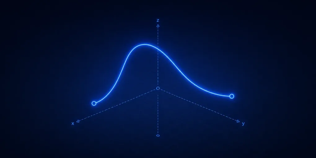
The visualization below shows one cubic 3D Bezier curve. The blue curve is sampled from many values of . The dashed brown segments connect the four control points. The moving construction chain shows how the current point is computed. Dragging the canvas rotates the camera, while the t slider moves the highlighted construction point along the curve.
The most important first observation is that rotation changes the drawing without changing the curve. Drag the canvas horizontally until the dashed polygon appears flatter, then rotate it back until the depth separation becomes visible again. The same four control points define the same spatial path the whole time. Only the projected view changes.
This distinction matters whenever a 3D curve is edited on a 2D screen. A handle that appears close to the curve may be far in depth. Two segments that appear to cross may only overlap after projection. A bend that looks mild from the front may become a deep S-shaped sweep from the side. The orbit interaction makes that ambiguity visible: the screen image is evidence about the curve, not the curve itself.
The grid and colored axes provide orientation cues. When a control point seems to move toward the viewer after rotation, it is not being edited; the camera is revealing the existing z placement. This is the key difference from a flat Bezier editor. In 3D, understanding the control polygon requires reading its shape from more than one viewpoint.
De Casteljau Works The Same Way In 3D
The cubic formula is concise, but the construction chain is usually easier to reason about. De Casteljau’s algorithm evaluates the curve by repeated linear interpolation. For a cubic curve, the first round interpolates along the three polygon edges:
The second round interpolates between those new points:
The final round interpolates once more:
Every step is just “move the same fraction along a segment.” That is why the algorithm is dimension-independent. If the endpoints are 3D points, each interpolation produces another 3D point. The method does not need a separate spatial trick.
In the visualization, scrub t slowly from 0 toward 1. Near t = 0, all intermediate points collapse toward . Near t = 1, they collapse toward . Around the middle, the chain spreads across the control polygon and the green point lands on the blue curve. The construction is not an approximation to the formula; it computes the same curve point by geometric blending.
The Michigan Tech page on De Casteljau’s algorithm is useful because it shows this interpolation ladder directly. The important extension here is that the ladder lives in space. When you orbit the view while keeping the same t, the intermediate points remain attached to the same 3D segments, but their screen layout changes with the camera.
Samples Turn The Continuous Curve Into A Drawing
The mathematical curve contains infinitely many points because can be any real value between and . A canvas, mesh, or rendering pipeline cannot draw infinitely many positions. It samples the curve at a finite set of parameter values and connects or displays those samples.
The small blue dots show that approximation. They are not control points. They are evaluated curve positions at regular intervals of . More samples make the drawn path look smoother, but they do not change the underlying curve. Fewer samples can make a curved path look like a broken polyline, especially where curvature changes quickly.
This is why de Casteljau and sampling solve different problems. De Casteljau answers “where is the exact curve point for this t?” Sampling answers “which evaluated points should we draw so the curve appears smooth enough?” A renderer may evaluate the curve many times, adaptively subdivide it, or split it into smaller pieces. Those are implementation choices built on the same geometric definition.
The broad WPI curve-generation notes make the same dimensional point in a compact way: adding a third coordinate equation is enough to move a parametric curve into 3D. The practical cost is not the definition; it is deciding how to display, sample, edit, and interpret that path in a projected view.
The Handles Shape Tangents And Depth
For a cubic Bezier curve, the first handle controls how the curve leaves , and the second handle controls how it approaches . More precisely, the endpoint tangent directions are proportional to these differences:
In 3D, those tangent vectors include depth. A handle can pull the curve upward, sideways, forward, or backward at the same time. From one camera angle, the start tangent may look mostly horizontal. After orbiting the view, the same tangent may reveal that it also points strongly along the depth axis.
The control polygon is helpful because it exposes those tangent relationships. The first dashed segment from to previews the departure direction. The last dashed segment from to previews the arrival direction. The curve does not trace those segments, but it uses them to decide how to leave and enter the endpoints.
This is one reason 3D Bezier curves are useful for camera rails and object motion. The curve gives a smooth position path, while the tangent gives a local direction of travel. That does not automatically solve orientation. A camera or object following a spatial curve still needs a rule for roll, up direction, or frame construction. The curve tells you where the object is and where it is heading; the application decides how it should face.
Projection Can Hide Real Curve Shape
Because the final image is projected onto a 2D screen, different 3D curves can sometimes look similar from one view. This is not a Bezier-specific problem. It is a general property of 3D visualization. The solution is to use depth cues, rotate the view, and keep the control polygon visible.
In the visualization, place t near the middle and rotate the camera until the green construction point appears close to one of the dashed polygon segments. Then rotate again. The apparent closeness changes because the screen distance is not the full 3D distance. What looked like a near contact in projection may separate clearly once depth is visible.
This is also why a 3D Bezier editor usually needs multiple views, snapping modes, or explicit coordinate controls. Dragging a point freely in screen space is ambiguous unless the tool defines which plane or axis receives the edit. The article’s visualization does not edit the control points, but the same ambiguity appears while merely reading the curve: a single projection cannot tell the whole spatial story.
Curves Lead Naturally To Surfaces
3D Bezier curves are often a stepping stone toward Bezier surfaces. A curve uses one parameter, . A tensor-product Bezier surface uses two parameters, often written and , and a grid of control points. Holding one parameter fixed gives a curve across the surface. The Wellesley notes on Bezier surfaces and 3D shapes explain this graphics connection by showing how surface edges and interior control points shape a patch.
That extension is important, but it is not required for understanding the curve in this article. The curve already contains the main ideas: control points define a geometric scaffold, interpolation turns that scaffold into a smooth path, and projection determines how the 3D result appears on a flat screen. Surface patches reuse those ideas with a richer control net.
For deeper practical curve handling, including subdivision, derivatives, curve fitting, and many implementation details, A Primer on Bezier Curves is the best next reference. Its breadth is useful after the core spatial model is clear, especially if you are building tools that need splitting, measuring, offsetting, or projecting Bezier curves robustly.
The Core Mental Model
A 3D cubic Bezier curve is a smooth spatial path controlled by four points. The endpoints lie on the curve. The interior points pull the departure and arrival behavior. The parameter selects one point along the mathematical path. De Casteljau’s algorithm finds that point through repeated interpolation, and the same construction works because 3D points can be blended just like 2D points.
The part that becomes harder in 3D is not the formula. It is interpretation. The control polygon, sampled curve, and construction chain all live in space, but the screen shows a projection. Orbiting the view is therefore not cosmetic; it is part of understanding the geometry. Once that distinction is clear, 3D Bezier curves become a direct extension of the 2D curves used in vector graphics, with enough spatial control for motion paths, modeling guides, and surface boundaries.